In
this chapter, the materially coupled bending-torsion vibration of
laminated composite beam, based on an assembly of uniform beam elements,
and using the Finite Element Method (FEM), Dynamic Stiffness Matrix
(DSM) and Dynamic Finite Element (DFE) is presented. The DSM method is
based on the exact solution to the governing differential equations of
motion, as presented by Banerjee and Williams (1995). Therefore, for a
uniform beam, the DSM needs only one element to achieve the exact
natural frequencies. The DSM formulations can also be easily extended to
approximate tapered geometry by using a piece-wise uniform stepped
model. The FEM model is obtained using a Galerkin weighted residual
method to formulate the element mass and stiffness matrices of the
current uniform beam. In what follows, a Dynamic Finite Element method
for the coupled vibration analysis of uniform and stepped composite
beams is developed. The comparison is then made between the DFE results
and those obtained from the FEM and DSM formulations in order to
validate the proposed methodology.
A cantilever
composite beam with length L and a solid cross-section is the
basis of the model (see Figure 4-1). All rigidities are assumed constant
along y axis. The rigidities are: bending, EI, torsion,
GJ, and coupled bending-torsion, K. The rigidities can be
determined either experimentally or based on the theory presented in
Chapter 3. The solid cross section is assumed to be symmetric with different
fibre layer orientations (see Figure 4-1), where
 is the translational displacement associated with bending and
 is
the rotational twist associated with torsion.
is
the rotational twist associated with torsion.
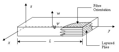
Figure 4-1:
Composite Beam on a Right Handed Coordinate System.
The
simplest model of a composite wing is represented by a uniform
Euler-Bernoulli beam, where the bending slope is the derivative of the
bending displacement with respect to the span-wise direction (Lilico
et al, 1997). Shear deformation and rotary inertia are neglected by
assuming a long slender beam. Further simplifications have been made by
applying the St. Venant assumptions, which is a pure torsion state, and
neglecting all warping effects. The beam is assumed to be composed of
composite material with unidirectional fibre lay-up. With any composite,
material couplings between extensional-twist and bending-twist arise
from ply orientation and stacking sequence. This research will focus on
the bending-twist couplings as the other coupling behaviours are being
investigated by other researchers (see, for example, Roach and Hashemi,
2003).
The governing differential equations of motion for
the materially coupled vibration of a uniform composite beam are
(Banerjee, 1998):
 (4.1)
(4.1)
 (4.2)
(4.2)
where denote
the beam flexural displacement and
denote
the beam flexural displacement and
 is
the torsion angle. EI and
GJ denote flexural and torsion rigidities respectively,
m is the mass per unit length and
is
the torsion angle. EI and
GJ denote flexural and torsion rigidities respectively,
m is the mass per unit length and
 represents
the polar mass moment of inertia per unit length of the wing. The
material bend-twist coupling rigidity is represented by K and
primes denote differentiation with respect to span wise position y.
Based on the simple harmonic motion assumption, the following separation
of variables is applied on the flexural and torsional displacements
(sinusoidal variation with frequency
represents
the polar mass moment of inertia per unit length of the wing. The
material bend-twist coupling rigidity is represented by K and
primes denote differentiation with respect to span wise position y.
Based on the simple harmonic motion assumption, the following separation
of variables is applied on the flexural and torsional displacements
(sinusoidal variation with frequency ).
).
 (4.3)
(4.3)
Then with substitutions of (4.3) into (4.1) and
(4.2), the differential equations can be re-written in the following
form:
 (4.4)
(4.4)
 (4.5)
(4.5)
By implementing the Galerkin weighted residual method and integration by
parts, the continuity requirements on the field variable are relaxed so
that the integral weak form associated with equations (4.4) and (4.5)
can then be obtained as:
 (4.6)
(4.6)
 (4.7)
(4.7)
The above
boundary terms can be associated with the Shear S(y), Moment
M(y), and torque T(y) as:
 (4.8)
(4.8)
 (4.9)
(4.9)
 (4.10)
Boundary conditions associated with clamped-free (cantilever) beam are
 ,
and all force boundary terms are zero at the tip (y=L). The
system is then discretized by 2-node 6-DOF beam elements (Figure 4-2).
,
and all force boundary terms are zero at the tip (y=L). The
system is then discretized by 2-node 6-DOF beam elements (Figure 4-2).
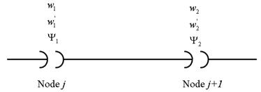
Figure 4‑2: A 2-node
6-DOF beam element
Principle of Virtual Work (PVW) is also satisfied such that:
 (4.11)
where,  represents
element internal virtual work and
represents
element internal virtual work and
 for
free vibrations. After two integrations by parts on the differential
equation governing the flexural motion, the element internal virtual
work can be written in the following form:
for
free vibrations. After two integrations by parts on the differential
equation governing the flexural motion, the element internal virtual
work can be written in the following form:
 (4.12)
where,
 (4.13)
and,
 (4.14)
The two above
equations simply represent the bending and torsion contributions to the
discretized internal virtual work for each element of length
 .
.
The basis functions are then chosen based on the solutions to the
differential equations of (*) and (**). For the first differential
equation (4.13) pertaining to bending, the following process is applied
to formulate the trigonometric shape functions according to Hashemi and
Richard (1999). The torsion interpolation functions are also evaluated
in a similar way.
The non-nodal
approximation for the flexural weighting function,
 ,
and the field variable,
,
and the field variable, ,
can be written as:
,
can be written as:
 (4.15)
Similarly for
torsion:
 (4.16)
where
dw,
w, are
discretized over a single element (0
are
discretized over a single element (0
 x
1).
The basis functions of the approximation space are chosen as:
x
1).
The basis functions of the approximation space are chosen as:
 (4.17)
and, for
torsion as:
 (4.18)
where,
 (4.19)
 (4.20)
The basis functions are chosen
as trigonometric terms based on the solution to the differential
equations and were manipulated to reduce to Hermitian basis functions as
 .
It is important to note that Hermitian basis functions have been used in
beam finite elements for many years, since they satisfy the
Completeness and Compatibility requirements. Completeness is
satisfied by including the lowest order admissible term. The
compatibility condition is also satisfied. With these conditions
satisfied, the DFE with its Hermitian based Dynamic Trigonometric Shape
Functions (DTSFs) is guaranteed to converge to the exact solution.
Classical basis functions of the standard Hermite beam element are [1,
x,
x2,
x3].
The bending and torsion trigonometric basis functions lead to standard
cubic and linear ones by taking the limit as
,
respectively. These variables are frequency dependent as seen above in
equations (4.19) and (4.20). When the frequency approaches zero the
DTSFs reduce to polynomial basis functions which lead to satisfying the
required conditions of compatibility and completeness.
.
It is important to note that Hermitian basis functions have been used in
beam finite elements for many years, since they satisfy the
Completeness and Compatibility requirements. Completeness is
satisfied by including the lowest order admissible term. The
compatibility condition is also satisfied. With these conditions
satisfied, the DFE with its Hermitian based Dynamic Trigonometric Shape
Functions (DTSFs) is guaranteed to converge to the exact solution.
Classical basis functions of the standard Hermite beam element are [1,
x,
x2,
x3].
The bending and torsion trigonometric basis functions lead to standard
cubic and linear ones by taking the limit as
,
respectively. These variables are frequency dependent as seen above in
equations (4.19) and (4.20). When the frequency approaches zero the
DTSFs reduce to polynomial basis functions which lead to satisfying the
required conditions of compatibility and completeness.
For the first
bending basis function:
 (4.21)
The second
basis function leads to:

 (4.22)
The third basis
function leads to:

 (4.23)
The fourth
basis function leads to:

 (4.24)
The coefficients have
no physical meaning and can be replaced by nodal variables for bending
have
no physical meaning and can be replaced by nodal variables for bending
 and
and
 and
for torsion
and
for torsion and
and
 .
The derivation of
bending shape functions are only considered in the following procedure,
since, the torsion shape functions will follow the same development.
Following the same systematic method as in FEM, one can write:
.
The derivation of
bending shape functions are only considered in the following procedure,
since, the torsion shape functions will follow the same development.
Following the same systematic method as in FEM, one can write:
 (4.25)
 (4.26)
Then,
 (4.27)
The nodal
approximations for element variables and
 can
then be rewritten as:
can
then be rewritten as:
 (4.28)
 (4.29)
Then,
 (4.30)
Expressions (4.30) can then be rearranged as:
 where
where
 is
the element displacements (i.e., degrees of freedom) and [N]
represents the dynamic shape functions in matrix form.
is
the element displacements (i.e., degrees of freedom) and [N]
represents the dynamic shape functions in matrix form.
 (4.31)
The four trigonometric shape functions pertaining to bending are
(Hashemi and Richard 1999; Hashemi, 1998):
 (4.32)
 (4.33)
 (4.34)
 (4.35)
 (4.36)
For torsion:
 (4.37)
 (4.38)
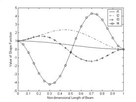
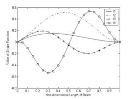
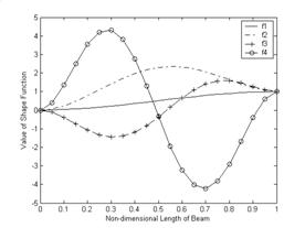
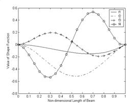
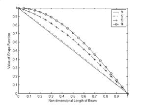
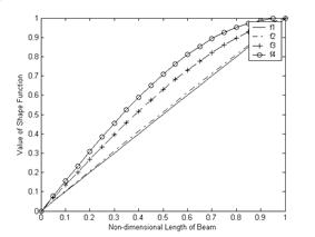
The
six shape functions are plotted individually for first four natural
frequencies of free coupled vibration of a uniform composite wing (see
Figures 4-3 through 4-8). These shape functions are the approximations
to the solution of the governing differential equations of motion.