The
materially coupled composite, uniform and piece-wise uniform stepped
wing beams were analysed in Chapter 4. The tapered wing configurations
were then presented and discussed in Chapter 5. In this chapter, the
wing model is extended to more complex configurations exhibiting not
only the material but also geometrical couplings. Using a wing-box model
for the wing cross-section and a circumferentially asymmetric stiffness
(CAS) configuration for the composite ply lay-up, a more realistic
composite wing model is generated. In the previous chapters, only
material coupling was considered which arises from an unbalanced ply
lay-up or symmetric stacking sequence. An additional geometric coupling
arises from the cross-sectional geometry of the wing.
The present wing model, (Figure 6‑2(a))
is modeled as a symmetric configuration where the materially coupled
behaviour is characterized by bending-torsion coupled stiffness K.
The added geometric coupling is a consequence of an offset of the
mass centre axis, Gs, from the geometrical elastic axis, Es,
denoted by xα. Any structural component located in
front of the leading spar or behind the rear spar is considered not to
contribute to the rigidity of the wing (Lillico, Butler, Guo and
Banerjee, 1997). The omitted components do however contribute to the
mass and inertia of the wing such that the mass centre, initially
located at the geometric centre of the box, shifts slightly towards the
rear of the wing-box (refer to Figure 6‑2(b)).
The
proposed wing model is constructed as a wing-box, where L is the
span-wise length and c is the wing chord. The lateral bending and
twist displacements are governed by Euler-Bernoulli and St. Venant beam
theories, respectively. Shear deformation, rotary inertia, commonly
associated with Timoshenko beam theory, as well as warping effects are
neglected.
Different stacking sequence and/or thickness of the thin-walled box-beam
result in different coupling behaviours. For a circumferentially
asymmetric stiffness (CAS) configuration the axial stiffness, A,
must remain constant in all walls of the cross-section. The coupling
stiffness, B, in opposite members is of the opposite sign as
stated by Armanios and Badir (1995) and Berdichevsky et al (1992).
As a result of axial stiffness, A, remaining constant, the
corresponding thickness must also remain constant. Chandra et al.
(1990) consider a symmetric configuration for a box-beam which consists
of opposite walls having the same stacking sequence, although the
stacking sequences between the horizontal and vertical members need not
be the same. The CAS and symmetric configurations both lead to a
bending-torsion coupled response for thin-walled beams.
The second configuration considered by Armanios and Badir (1995) and
Berdichevsky et al (1992) was a circumferentially uniform
stiffness configuration (CUS) where A, B, C, axial, coupling and
shear stiffness, respectively, are constant throughout the circumference
of the cross-section. Chandra et al. (1990) built-up similar
configurations where the stacking sequence of opposite walls is of
oppositely stacked, what they call anti-symmetric configuration.
Anti-symmetric or CUS configurations are beyond the scope of this
research and will not be discussed further. The CAS or symmetric
configuration leads a bending-torsion coupled wing which will be used to
model the wing-box composite plies.
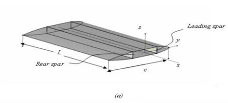
Figure 6‑1: (a) 3-D drawing of a
composite wing cross-section airfoil, with length = L.
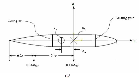

Figure
6‑2: (b) Cross-section of
a wing-box, where c is the chord length, Mbox
is the wing-box mass, Es and Gs are,
respectively, the geometric elastic centre and mass centre axis.
6.3
Theory
The
differential equations governing the motion for the free vibration of
laminated composite wings (presented in Figures 6-1(a, b)) with
geometric couplings are given by Lillico et al (1997) as:
 (6.1)
(6.1)
 (6.2)
(6.2)
The
displacements can be assumed to have a sinusoidal variation with
frequency as:
as:
 (6.3)
(6.3)
The Weighted Residual Method (WRM)
is employed and the integral form is re-written in the following weak
form
 (6.4)
(6.4)
 (6.5)
(6.5)
where two integrations by parts for the flexural portion
and one integration by parts for the twisting portion have been applied.
Similar to Chapter 5, by re-writing the integral equation the
inter-element continuity requirements are relaxed so that once again the
approximation spaces for w and
f satisfy
the C1 and C0 continuity
requirements, respectively. Then, the resulting shear force, S(x),
bending moment, M(x), and torsional moment, T(x), are:
 (6.6)
(6.6)
 (6.7)
(6.7)
 (6.8)
(6.8)
The
sign conventions are similar to those already used in Chapters 4 and 5.
Boundary conditions associated to clamped-free (cantilever) structure
are such that all virtual and real
displacements are zero at wing root (x=0) and all
resulting forces are equal to zero at wing tip (x=L).
Hence,
 (6.9)
(6.9)
Consequently,
 (6.10)
Expressions (6.4) and (6.5) also
satisfy the Principle of Virtual Work (PVW) similar to formulation in
Chapter 5. The system is then discretized by 2-node 6-DOF uniform beam
elements over the length of the beam. The wing can be discretized to a
local domain  (i.e.,
reference element)
where,
(i.e.,
reference element)
where,  .
The uniform element virtual work expressions for bending and torsion
contributions can then be written as:
.
The uniform element virtual work expressions for bending and torsion
contributions can then be written as:
 (6.11)
and
 (6.12)
The
coupling terms in equations (6.11) and (6.12) are equivalent and when
written in matrix form they are only different by their dimensions. The
coupling terms in the weak form retain symmetry of the final element DFE
matrix. The DFE takes the average over each element (similar to the DSM)
for EI( ),
m(),
GJ(),
),
m(),
GJ(),
 and K().
Therefore, after a certain number of additional integration by parts,
the expressions for flexural and twist are found as:
and K().
Therefore, after a certain number of additional integration by parts,
the expressions for flexural and twist are found as:
 (6.13)
and,
 (6.14)
such
that,
 (6.15)
The
Dynamic Trigonometric Shape Functions (DTSFs) are then defined such
that the integral expressions
 and
and are
zero. The variable mechanical properties are averaged differently
compared to the previous models developed. The following integral
averaging technique is employed to allow for flexibility in the model,
are
zero. The variable mechanical properties are averaged differently
compared to the previous models developed. The following integral
averaging technique is employed to allow for flexibility in the model,
 (6.16)
so
that the dually coupled wing-beam, exhibiting material and geometric
couplings, can be easily extended to higher order taper configurations.
 can
be any mechanical property varying along the wing span (refer to Figure
6-2).
can
be any mechanical property varying along the wing span (refer to Figure
6-2).
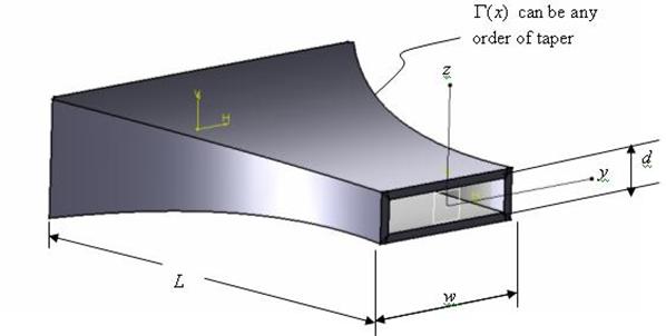
Figure
6‑3 :
: Dually tapered composite wing-box
:
: Dually tapered composite wing-box
Finally, the approximations to the field and test variable w,
 ,
,
 and
and
 are
substituted into the above equations and the corresponding DFE matrices
are obtained as:
are
substituted into the above equations and the corresponding DFE matrices
are obtained as:

(6.17)
 (6.18)
 (6.19)
Similar to equation (5.18) and (5.19) deviator expressions can also be
added to refine the dynamic stiffness matrix RDFE to incorporate
variable mechanical and/or geometric parameters:
 (6.20)
 (6.21)
The
only major difference between equations (6.20) and (6.21) and equations
(5.18) and (5.19) is an added bending-torsion coupling associated with
 term.
The deviator matrices are then constructed in the same way leading to:
term.
The deviator matrices are then constructed in the same way leading to:
 (6.22)
where,
 (6.23)
Due to the unavailability a closed form symbolic integration for the
deviator terms. The deviator terms rely on a numerical 16 point gauss
quadrature integration.
Numerical Free Vibration Results
Wittrick-Williams root
counting algorithm
